
Google Sheets QUERY Reports with Dropdown Filters
To build a filtered report in Google Sheets, use QUERY: =QUERY(data, "query", 1). The query string is made of clauses such as select, where, group by, pivot, order by, label and format, and the last argument is the number of header rows. For a report that others can filter, put a region dropdown and two date cells on a separate tab, and join those cells into the query string with &. The biggest trap is that QUERY can return an incomplete result without any error: a single date stored as text drops that order from the report silently.
The limit is clear from the start: everyone with access sees the same file, rows can’t be hidden per person, and the report is a copy of its source.
How is QUERY written, and what changes with the locale?
QUERY takes three arguments: the range to query, the query string in quotation marks, and the number of header rows at the top of the range. Google’s QUERY help page gives the syntax as QUERY(data, query, [headers]). If headers is omitted, Google guesses it from the content. I always write 1.
According to the query language reference, clauses must appear in this order:
select: which columns (select A, C, F)where: which rows (where C = 'West')group by: grouping, with aggregates such assum(F)orcount(A)pivot: values of one column become new columnsorder by: sorting (order by sum(F) desc)limit,offsetlabel: renaming result headersformat: formatting result values
Keywords are case-insensitive, but identifiers and string literals are case-sensitive: 'Cancelled' and 'cancelled' are different values. In the Turkey-locale test, the equivalent lower-case query raised no error and found no rows.
Separators. The locale lives under File > Settings. US-locale files separate arguments with commas; my US test file also converted a semicolon formula to commas. Some locales, Turkey for example, use semicolons. Commas inside the query string (select A, B) stay commas everywhere, because quoted text is a query, not a formula. When pasting a tutorial from another locale, change only the separators outside the quotes.
In Turkey. In a Turkey-locale test file, the comma version failed with “Formula parse error” and the semicolon version worked; Google’s Turkish help page also writes the syntax with semicolons. Most tests below were run in that file.
Function names. The formulas use English names; their language is a separate setting (“Always use English function names”, Google).
Example: a regional order report at a distributor
The company, customer codes and figures are fictional.
An industrial distributor sells bearings, belts and chains through four regional sales teams: North, West, South and Central. Orders live in one Google Sheets file, on an Orders tab. Columns: A Order No, B Date, C Region, D Customer, E Product, F Amount (net), G Status (Open, Shipped, Cancelled). The tab holds 28 orders dated between 2026-07-01 and 2026-08-07.
The sales manager’s question: between 2026-07-01 and 2026-07-31, excluding cancellations, how many orders and what total per region? Four of the rows:
| No | Date | Region | Amount | Status |
|---|---|---|---|---|
| 1009 | 2026-07-13 | Central | 40,150 | Shipped |
| 1010 | 2026-07-14 | West | 7,350 | Cancelled |
| 1011 | 15.07.2026 (text) | West | 41,200 | Shipped |
| 1012 | 2026-07-16 | South | 11,200 | Shipped |
The date for 1011 was pasted as plain text from another file; Sheets stores it as text.
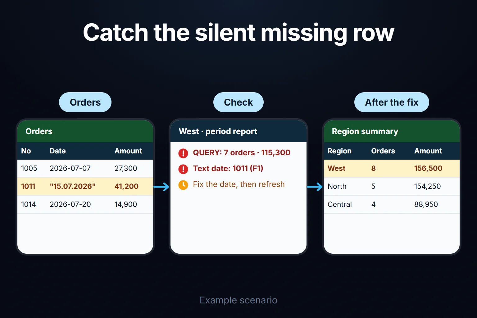
The West manager picks West. QUERY shows 7 orders, 115,300. In fact the period has 8 orders, 156,500 that weren’t cancelled. The gap is one row, 1011, worth 41,200, and the report shows no warning.
That gap changes a decision. The regional summary puts North first at 154,250 and West second at 115,300; with 1011 fixed, West leads with 156,500. A manager setting bonuses or stock priority from this table would favour the wrong region.
On 16 October 2026 I built this example in real Google Sheets files (Turkey and United States locales), entered the formulas through the Sheets API and read the results back. A Python script mimicking QUERY’s logic gave the same figures.
How do you build the report tab step by step?
The report tab is a few input cells plus the QUERY formulas that read them; nobody types data into it. The layout:
Report!B1Region (dropdown),B2Start date,B3End date,B4Customer (for the apostrophe example)A6filtered order list,H6regional summary,H13region × product tableD1andF1check cells
1. Dropdown and date cells
On a separate Settings tab, type the four regions and “All” into A2:A6. Select B1 and use Insert > Dropdown or Data > Data validation, choosing “Dropdown (from a range)” and pointing to that range (Google Help, read 16 October 2026). Google says an entry that doesn’t match the list is rejected by default, so a typo such as “Wset” never reaches the report.
Enter real dates in B2 and B3; right alignment shows Sheets recognised them.
2. Filtered list: taking criteria from cells
Report!A6:
=QUERY(Orders!A1:G,"select A, B, E, F, G where G <> 'Cancelled' and B >= date '"&TEXT(B2,"yyyy-mm-dd")&"' and B <= date '"&TEXT(B3,"yyyy-mm-dd")&"' and C = '"&B1&"' order by B",1)In '"&B1&"' the single quotes belong to the query, the double quotes to the formula, and & inserts the cell value.
Dates are stricter. The query language accepts a date only as date 'yyyy-MM-dd'. TEXT(B2,"yyyy-mm-dd") converts the cell into that form; the format code uses these English letters even in the Turkey-locale file. Read back on its own, it produced 2026-07-01 in both test files.
Result:
| No | Date | Product | Amount | Status |
|---|---|---|---|---|
| 1002 | 2026-07-02 | Belts | 12,650 | Shipped |
| 1005 | 2026-07-07 | Bearings | 27,300 | Shipped |
| 1007 | 2026-07-09 | Chains | 9,800 | Shipped |
| 1014 | 2026-07-20 | Chains | 14,900 | Shipped |
| 1017 | 2026-07-23 | Bearings | 21,450 | Open |
| 1020 | 2026-07-28 | Belts | 10,900 | Open |
| 1023 | 2026-07-31 | Bearings | 18,300 | Open |
1010 is missing because it was cancelled, which is correct. 1011 is missing by mistake.
3. Regional summary: GROUP BY, ORDER BY, LABEL, FORMAT
The summary and pivot deliberately show every region and ignore B1. Report!H6:
=QUERY(Orders!A1:G,"select C, count(A), sum(F) where B >= date '"&TEXT(B2,"yyyy-mm-dd")&"' and B <= date '"&TEXT(B3,"yyyy-mm-dd")&"' and G <> 'Cancelled' group by C order by sum(F) desc label C 'Region', count(A) 'Orders', sum(F) 'Amount' format sum(F) '#,##0'",1)| Region | Orders | Amount |
|---|---|---|
| North | 5 | 154,250 |
| West | 7 | 115,300 |
| Central | 4 | 88,950 |
| South | 3 | 69,800 |
Without label, headers read “count Order No” and “sum Amount”. In '#,##0' the comma means thousands separator, so the display follows the locale: 154,250 in the US file, 154.250 in the Turkey file. The total is 19 orders and 428,300. With 1011 fixed it should be 20 orders and 469,500.
4. Region × product: PIVOT
Report!H13:
=QUERY(Orders!A1:G,"select C, sum(F) where B >= date '"&TEXT(B2,"yyyy-mm-dd")&"' and B <= date '"&TEXT(B3,"yyyy-mm-dd")&"' and G <> 'Cancelled' group by C pivot E",1)| Region | Bearings | Belts | Chains |
|---|---|---|---|
| Central | 40,150 | 8,600 | 40,200 |
| North | 101,000 | 28,650 | 24,600 |
| South | 58,600 | 11,200 | (blank) |
| West | 67,050 | 23,550 | 24,700 |
pivot implies aggregation, so sum(F) and group by C go with it. Product columns opened alphabetically. South’s only chain order (1016) was cancelled, so that cell is blank, not zero. West’s bearings total shows 67,050 because of 1011; fixed, it would be 108,250.
5. An “All” option
The list formula in step 2 returns nothing when “All” is selected, because no row’s region is “All”. Replace this piece inside the formula:
and C = '"&B1&"'with this:
"&IF(B1="All",""," and C = '"&B1&"'")&"With “All” in B1 the region condition disappears; with any other value it is added. I ran the modified formula in the Turkey-locale file in both branches: “All” returned 19 orders from four regions, and the single region returned the 7 rows above.
6. Check cells: making the silent error visible
QUERY skips bad data without warning, so I put two checks next to the report. Report!D1 counts text cells in the date column, and Report!F1 lists their order numbers:
=SUMPRODUCT(--ISTEXT(Orders!B2:B))
=IFERROR(FILTER(Orders!A2:A,ISTEXT(Orders!B2:B)),"None")
In the test D1 returned 1 and F1, with IFERROR, showed 1011. Above zero, the report is incomplete. I didn’t test the “None” branch, since the data always had a text date. Add the same check for amounts with ISTEXT(Orders!F2:F).
Fixing text dates. Re-enter a single cell as a date, or use DATEVALUE: in the Turkey-locale file both DATEVALUE("15.07.2026") and a cell reference returned the right date. To fix hundreds of rows, put this in an empty column, then paste the result back over column B as values:
=ARRAYFORMULA(IF(Orders!B2:B29="","",IF(ISTEXT(Orders!B2:B29),DATEVALUE(Orders!B2:B29),Orders!B2:B29)))In the test all 28 rows became date serials, 1011 included. Adjust the range and apply a date format.
What if a criterion cell is text? With the start date typed as plain text in a test cell, TEXT still produced 2026-07-01 and the query worked: Sheets converted a date string it recognised. I didn’t test unrecognisable text; date validation on B2 and B3 reduces the risk.
What if nothing matches? QUERY returns just the header row, not an error, so IFERROR didn’t catch it in my test. Check the row count instead:
=IF(ROWS(QUERY(Orders!A1:G,"select A where C = 'East'",1))<2,"No records",QUERY(Orders!A1:G,"select A where C = 'East'",1))In the Turkey-locale file it showed “No records” for a missing region and the list for an existing one. The query appears twice; edit both copies together.
Thousands of rows? These measurements used 28 orders. I haven’t measured how QUERY performs on tens of thousands of rows.
Common QUERY errors and their causes
Half of QUERY’s problems show up as errors, half as missing or empty results. I reproduced all eight in the Turkey-locale test file (formulas differ only in separators): seven as described, the #N/A case with an array, not IMPORTRANGE:
| Symptom | Cause | Fix |
|---|---|---|
| “Formula parse error” | Commas used as separators in a semicolon locale | Change separators outside the quotes |
| #VALUE!, “Invalid date literal” | Date written as date '01.07.2026' | date 'yyyy-MM-dd', or TEXT(B2,"yyyy-mm-dd") from a cell |
| No error, empty result | Date compared with a string, no date keyword (B >= '2026-07-01') | Add date to the comparison |
| No error, missing rows | Mixed data types in a column: a text date or text amount | Check cells, fix at source |
| #N/A | Column letters used on an array (not tested with IMPORTRANGE) | Col1, Col2 notation |
| #VALUE!, “PARSE_ERROR” | Criterion from a cell contains an apostrophe (MK'101) | Wrap the criterion in double quotes |
| No error, count blank instead of zero | Text case doesn’t match ('cancelled' vs Cancelled) | Pick values from a dropdown |
| Result runs to the end of the sheet | An open range also returns blank rows | Add where A is not null |
Mixed data types. Google’s QUERY page states the rule: with mixed data types in one column, the majority type determines the column’s type and minority types are treated as null. Here the date column holds 27 dates and one text value, so the text became null and fell outside every date range; select A, B, F where A = 1011 returned an empty date. An amount typed as text may appear in a list but won’t be added to a total.
Apostrophes and quotes. The reference allows string literals in single or double quotes. If a cell value contains an apostrophe (MK'101, 3/4'' hose, O'Brien), a single-quoted query string breaks at that point; in the test it returned “PARSE_ERROR”. Wrap the criterion in double quotes inside the query; in a formula, one double quote is written as two. With the customer criterion in B4:
=QUERY(Orders!A1:G,"select A where D = """&B4&"""",1)This version ran without error. If the value itself contains a double quote, clean that out instead. A dropdown avoids both problems.
Date and time. If the date column also holds times, the query language uses datetime 'yyyy-MM-dd HH:mm:ss'. The example has no times, and I didn’t test this.
Blank rows. An open range such as Orders!A1:G includes every empty row. An unfiltered select A, C returned 1,000 rows in the test file; where A is not null cut it to 29 (header plus 28 orders).
Arrays, IMPORTRANGE and QUERY: why Col1?
When the data given to QUERY was an array ({Orders!A1:G}), column letters failed and positional names worked: select C, sum(F) returned #N/A, while select Col3, sum(Col6) ... group by Col3 returned the right totals. Google’s QUERY page only says both notations are accepted. An IMPORTRANGE result is also an array from another file rather than a plain range, so I use Col notation there too, but I couldn’t test IMPORTRANGE through the API, because the file connection is approved in the interface (“Allow access”). In a regional file:
=QUERY(IMPORTRANGE("source-file-url","Orders!A1:G"),"select Col1, Col2, Col4, Col6 where Col3 = 'West'",1)Google’s IMPORTRANGE page says the function checks for updates every hour while the document is open (read 16 October 2026). Once several files depend on each other, tracking which source refreshed when becomes a job in itself; I cover that on the central data portal page.
Where does this report stop being enough in Google Sheets?
A QUERY report is enough as long as everyone who opens it may see every order. If the West manager should see only West, Sheets can’t enforce that split reliably. There are three limits.
Everyone sees the same file. Sharing works at file level, and picking West in a dropdown is a view, not a permission. Google’s protection help says hiding a sheet is not the same as protecting it, and viewers can still access content in hidden sheets. About protected ranges, Google writes: “This shouldn’t be used as a security measure.” People can copy, print and export a protected spreadsheet.
One file per region doesn’t hide rows either. The obvious workaround is a file per region pulling only that region with IMPORTRANGE and QUERY. According to Google’s IMPORTRANGE page, once access is granted, any editor of the destination file can pull from any part of the source. Someone with edit rights to the West file can change the formula and pull North’s orders. Share the regional file as view-only and the regional manager can no longer enter anything.
The report is a copy of its source. QUERY reads data; it doesn’t fix it, and it doesn’t show who changed the source, when or why. With four regional files, each is an hourly copy, and a mistake at the source reaches all four.
If nobody needs a per-person split, the setup above is enough and easy to maintain.
Where does a role- and permission-based app begin?
A role- and permission-based app begins when different people must see different rows of the same report, and that split must not be bypassable. A decision table:
| Your situation | My recommendation | Why |
|---|---|---|
| Every reader may see every region; one or two people enter data | Sheets + QUERY | Nothing to hide; the check cells catch silent errors |
| Every reader may see everything; each region enters its own orders | Sheets with dropdowns and data validation | Fewer entry errors, no permission problem |
| Each regional manager may see only their own region, or changes must be traceable | Role- and permission-based app | Row-level separation and a change log can’t be enforced reliably in Sheets |
In the first two rows, this page’s setup does the job: what closes the 41,200 gap is a check cell, not an app.
In an app, permission can be built as a query rule, not hidden screen content: the West manager’s request returning only West’s rows, as on the assigned-records tracking portal. The sales manager sees all regions. The rule I suggest: nobody approves the cancellation of an order they entered. A defined business rule is applied as data is entered: the date field can be set to reject text, so a row like 1011 doesn’t arise.
AI. Every figure comes from a defined query; the model doesn’t produce numbers. It can suggest explanations, such as “the largest West order in the period is 41,200”. The app can be set up so that no row reaches the model without passing the permission filter, so each manager’s explanation is built only from rows that person may see.
Delivery. The app runs on a server (VPS) that can be opened in your company’s name. The data is yours, exportable as Excel or CSV at any time. For a small or mid-sized team there are no per-user licence fees; the cost is the server plus maintenance. The source code sits in a repository you can access, with run instructions, a dependency list and known limits. Scope is set in writing in the first step. More examples are on the custom web apps for your team page.
What happens to the data in Sheets? The orders tab is imported. The rule I suggest: text dates and amounts go to a separate list and aren’t loaded until fixed, so 1011 is corrected there first. Your report tab stays as a cross-check against the app’s summary.
Send a copy of your report tab through the contact page. In the first meeting we’ll look at which rows are dropping out of it silently, and whether you need a per-person split at all.
Frequently Asked Questions
Does FILTER avoid this trap?
No. In the Turkey-locale test file I ran FILTER with the same region and date conditions: it also dropped 1011 and returned 7 orders totalling 115,300. FILTER compares dates directly with the cell, without the date keyword. If you need grouping, sorting and renamed headers, QUERY is shorter. Either way, you need the check cells. I didn’t test a pivot table on this data.
What happens if I type over a QUERY result?
The whole formula breaks. In the test, a note typed into one cell of the list area turned the formula into #REF! and the list disappeared: the result won’t spill over a cell that holds data. Keep notes in a column beside the result, or paste the result as values on another tab and record the date of the copy.
Can I ask an AI assistant to write the QUERY formula?
Yes. Give it the column letters, your locale and the criteria cells, and the draft usually has the right structure. But the model can’t see that one date is stored as text. Add the check cells and compare the result with a hand-counted total for one region.
How do I work?
Work-hour packages
Tell me about your business and what you need on WhatsApp or by phone; we agree on a work block of somewhere between 5 and 40 hours and I start doing what is needed. What you get is not a calendar window — it is net working hours spent directly on your business. I can use 40 hours working three days straight, or deliberately spread it out and finish it over a year — whatever the work calls for. I do not spend my time estimating how long something will take, I spend it doing the work; every hour I spend leaves a lasting result in your business. We keep going for as long as you find it useful.
Why not monthly?
Is 40 hours a week?
On a fixed monthly fee both sides are watching the wrong thing: you watch a fixed cost, the other side watches how many more contracts like this they can line up. Working by the hour puts us both in front of the same thing — the real value of the work that got done. I know not having an upfront answer to "how much will this cost in total?" is the natural cost of this model. But instead of paying a fixed fee for months to a setup that is not producing results, you only pay for the qualified time spent on your work — and you see exactly where that time went, start to finish. That is why my clients keep coming back.